PDBe search - with answers
This notebook is the second in the training material series, and focuses on getting information for multiple PDB entries using the REST search API of PDBe.
1) Making imports and setting variables
First, we import some packages that we will use, and set some variables.
Note: Full list of valid URLs is available from https://www.ebi.ac.uk/pdbe/api/doc/
[1]:
import requests # used for getting data from a URL
from pprint import pprint # pretty print
import matplotlib.pyplot as plt # plotting results
import pandas as pd # used for turning results into mini databases

# make graphs show on the page
%matplotlib inline

# use plotly and cufflinks to make interactive plots
import cufflinks as cf
from plotly.offline import download_plotlyjs, init_notebook_mode, plot, iplot
init_notebook_mode(connected=True)
cf.go_offline()


# settings for PDBe API
base_url = "https://www.ebi.ac.uk/pdbe/" # the beginning of the URL for PDBe's API.

api_base = base_url + "api/"

search_url = base_url + 'search/pdb/select?' # the rest of the URL used for PDBe's search API.
2) a function to get data from the search API
Let’s start with defining a function that can be used to GET data from the PDBe search API.
[2]:
def make_request(search_term, number_of_rows=10):
    """
    This function can make GET requests to
    the PDBe search API

    :param url: String,
    :param pdb_id: String
    :return: JSON
    """
    search_variables = '&wt=json&rows={}'.format(number_of_rows)
    url = search_url+search_term+search_variables
    print(url)
    response = requests.get(url)

    if response.status_code == 200:
        return response.json()
    else:
        print("[No data retrieved - %s] %s" % (response.status_code, response.text))

    return {}
3) formatting the search terms
This will allow us to use human readable search terms and this function will make a URL that the search API can handle.
[3]:
def format_search_terms(search_terms, filter_terms=None):
    # print('formatting search terms: %s' % search_terms)
    search_string = ''
    filter_string = ''
    search_list = []
    if isinstance(search_terms, dict):
        for key in search_terms:
            term = search_terms.get(key)
            if ' ' in term:
                if not '"' in term:
                    term = '"{}"'.format(term)
                elif not "'" in term:
                    term = "'{}'".format(term)
            search_list.append('{}:{}'.format(key, term))
        search_string = ' AND '.join(search_list)
    else:
        if '&' in search_terms:
            search_string = search_terms.replace('&', ' AND ')
        else:
            search_string = search_terms
    if filter_terms:
        filter_string = '&fl={}'.format(','.join(filter_terms))
    # print('formatted search terms: %s' % search_string)
    final_search_string = 'q={}{}'.format(search_string, filter_string)
    return final_search_string
4) Getting useful data out of the search
This function will run the search and will return a list of the results
[4]:
def run_search(search_terms, filter_terms=None, number_of_rows=100):
    search_term = format_search_terms(search_terms, filter_terms)

    response = make_request(search_term, number_of_rows)
    results = response.get('response', {}).get('docs', [])
    print('Number of results for {}: {}'.format(','.join(search_terms.values()), len(results)))
    return results
5) running a search
Now we are ready to actually run a search against the PDB API for entries containing human Dihydrofolate reductase in the PDB. This will return a list of results - only 10 to start with.
A list of search terms is available at: https://www.ebi.ac.uk/pdbe/api/doc/search
This will return details of human Dihydrofolate reductase’s in the PDB
The search terms are defined as a dictionary (a hash in other programming lanuguages). e.g. {“molecule_name”:“Dihydrofolate reductase”} Here we are searching for molecules named Dihydrofolate reductase. If we search for two terms i.e. molecule_name and organism_scientific_name then we will get molecules that match both search terms.
We will return the number of results for two searches.
The first one will hit the limit of 100. There are more than 100 Dihydrofolate reductase structures. We have to add the argument “number_of_rows” to a higher number, say 1000, to find all the examples.
[5]:
print('1st search')
search_terms = {"molecule_name":"Dihydrofolate reductase"}

results = run_search(search_terms)
1st search
https://www.ebi.ac.uk/pdbe/search/pdb/select?q=molecule_name:"Dihydrofolate reductase"&wt=json&rows=100
Number of results for Dihydrofolate reductase: 100
[6]:
results = run_search(search_terms, number_of_rows=1000)
https://www.ebi.ac.uk/pdbe/search/pdb/select?q=molecule_name:"Dihydrofolate reductase"&wt=json&rows=1000
Number of results for Dihydrofolate reductase: 365
We will add organism_name of Human to the query to limit the results to only return those that are structures of Human Dihydrofolate reductase.
[7]:
print('2nd search')
search_terms = {"molecule_name":"Dihydrofolate reductase",
                "organism_name":"Human"
               }
results = run_search(search_terms)
2nd search
https://www.ebi.ac.uk/pdbe/search/pdb/select?q=molecule_name:"Dihydrofolate reductase" AND organism_name:Human&wt=json&rows=100
Number of results for Dihydrofolate reductase,Human: 79
We will then look at the last result. We will print the data we have for the first result.
This will be the first item of the list “results” i.e. results[0]
We are using “pprint” (pretty print) rather than “print” to make the result easier to read.
[8]:
pprint(results[0])
{'_version_': 1656090036167245824,
'abstracttext_unassigned': ['Structural data are reported for the first '
'example of the potent antifolate inhibitor '
"2,4-diamino-5-methyl-6-[(3',4',5'-trimethoxy-N-methylanilino)methyl]pyrido[2,3-d]pyrimidine "
'(1) in complex with human dihydrofolate '
'reductase (hDHFR) and NADPH. Small differences '
'in crystallization conditions resulted in the '
'growth of two different forms of a binary '
'complex. The structure determination of an '
'additional crystal of a ternary complex of hDHFR '
'with NADPH and (1) grown under similar '
'conditions is also reported. Diffraction data '
'were collected to 2.1 A resolution for an R3 '
'lattice from a hDHFR ternary complex with NADPH '
'and (1) and to 2.2 A resolution from a binary '
'complex. Data were also collected to 2.1 A '
'resolution from a binary complex with hDHFR and '
'(1) in the first example of a tetragonal '
'P4(3)2(1)2 lattice. Comparison of the '
'intermolecular contacts among these structures '
'reveals differences in the backbone conformation '
'(1.9-3.2 A) for flexible loop regions (residues '
'40-46, 77-83 and 103-107) that reflect '
'differences in the packing environment between '
'the rhombohedral and tetragonal space groups. '
'Analysis of the packing environments shows that '
'the tetragonal lattice is more tightly packed, '
'as reflected in its smaller V(M) value and lower '
'solvent content. The conformation of the '
'inhibitor (1) is similar in all structures and '
'is also similar to that observed for TMQ, the '
'parent quinazoline compound. The activity '
'profile for this series of 5-deaza N-substituted '
'non-classical trimethoxybenzyl antifolates shows '
'that the N10-CH(3) substituted (1) has the '
'greatest potency and selectivity for Toxoplasma '
'gondii DHFR (tgDHFR) compared with its N-H or '
'N-CHO analogs. Models of the tgDHFR active site '
'indicate preferential contacts with (1) that are '
'not present in either the human or Pneumocystis '
'carinii DHFR structures. Differences in the '
'acidic residue (Glu30 versus Asp for tgDHFR) '
'affect the precise positioning of the '
'diaminopyridopyrimidine ring, while changes in '
'other residues, particularly at positions 60 and '
'64 (Leu versus Met and Asn versus Phe), involve '
'interactions with the trimethoxybenzyl '
'substituents.'],
'all_assembly_composition': ['protein structure'],
'all_assembly_form': ['homo'],
'all_assembly_id': ['1'],
'all_assembly_mol_wt': [22.497],
'all_assembly_type': ['monomer'],
'all_authors': ['Cody V', 'Gangjee A', 'Luft JR', 'Pangborn W'],
'all_compound_names': ['NDP : NADPH DIHYDRO-NICOTINAMIDE-ADENINE-DINUCLEOTIDE '
'PHOSPHATE',
'CO4 : '
'2,4-DIAMINO-5-METHYL-6-[(3,4,5-TRIMETHOXY-N-METHYLANILINO)METHYL]PYRIDO[2,3-D]PYRIMIDINE',
'CO4 : '
'5-methyl-6-{[methyl(3,4,5-trimethoxyphenyl)amino]methyl}pyrido[2,3-d]pyrimidine-2,4-diamine',
'CO4 : '
'5-methyl-6-[[methyl-(3,4,5-trimethoxyphenyl)amino]methyl]pyrido[3,2-e]pyrimidine-2,4-diamine',
'NDP : '
'[[(2R,3S,4R,5R)-5-(3-aminocarbonyl-4H-pyridin-1-yl)-3,4-dihydroxy-oxolan-2-yl]methoxy-hydroxy-phosphoryl] '
'[(2R,3R,4R,5R)-5-(6-aminopurin-9-yl)-3-hydroxy-4-phosphonooxy-oxolan-2-yl]methyl '
'hydrogen phosphate'],
'all_enzyme_names': ['Oxidoreductases',
'Acting on the CH-NH group of donors',
'With NAD(+) or NADP(+) as acceptor',
'Dihydrofolate reductase',
'1.5.1.3 : Dihydrofolate reductase',
'5,6,7,8-tetrahydrofolate:NADP(+) oxidoreductase'],
'all_go_terms': ['cytoplasm',
'mitochondrion',
'cytosol',
'folic acid binding',
'NADPH binding',
'oxidoreductase activity',
'RNA binding',
'sequence-specific mRNA binding',
'mRNA binding',
'methotrexate binding',
'NADP binding',
'dihydrofolate reductase activity',
'translation repressor activity, mRNA regulatory element '
'binding',
'drug binding',
'one-carbon metabolic process',
'folic acid metabolic process',
'negative regulation of translation',
'response to methotrexate',
'regulation of removal of superoxide radicals',
'tetrahydrobiopterin biosynthetic process',
'tetrahydrofolate biosynthetic process',
'tetrahydrofolate metabolic process',
'oxidation-reduction process',
'regulation of transcription involved in G1/S transition of '
'mitotic cell cycle',
'positive regulation of nitric-oxide synthase activity',
'axon regeneration',
'dihydrofolate metabolic process'],
'all_molecule_names': ['Dihydrofolate reductase', 'Dihydrofolate reductase'],
'all_num_interacting_entity_id': [0],
'all_sequence_family': ['IPR001796 : Dihydrofolate reductase domain',
'IPR017925 : Dihydrofolate reductase conserved site',
'IPR024072 : Dihydrofolate reductase-like domain '
'superfamily',
'PF00186 : DHFR_1',
'CL0387 : DHFred'],
'all_structure_family': ['3-Layer(aba) Sandwich',
'Alpha Beta',
'3.40.430.10',
'Dihydrofolate Reductase, subunit A',
'Dihydrofolate Reductase, subunit A',
'Alpha and beta proteins (a/b)',
'Dihydrofolate reductases',
'Dihydrofolate reductase-like',
'Dihydrofolate reductase-like'],
'assembly_composition': ['protein structure'],
'assembly_form': ['homo'],
'assembly_id': ['1'],
'assembly_mol_wt': 22.497,
'assembly_num_component': [1],
'assembly_type': ['monomer'],
'beam_source_name': ['Rotating anode'],
'biological_cell_component': ['cytoplasm', 'mitochondrion', 'cytosol'],
'biological_function': ['folic acid binding',
'NADPH binding',
'oxidoreductase activity',
'RNA binding',
'sequence-specific mRNA binding',
'mRNA binding',
'methotrexate binding',
'NADP binding',
'dihydrofolate reductase activity',
'translation repressor activity, mRNA regulatory '
'element binding',
'drug binding'],
'biological_process': ['one-carbon metabolic process',
'folic acid metabolic process',
'negative regulation of translation',
'response to methotrexate',
'regulation of removal of superoxide radicals',
'tetrahydrobiopterin biosynthetic process',
'tetrahydrofolate biosynthetic process',
'tetrahydrofolate metabolic process',
'oxidation-reduction process',
'regulation of transcription involved in G1/S '
'transition of mitotic cell cycle',
'positive regulation of nitric-oxide synthase activity',
'axon regeneration',
'dihydrofolate metabolic process'],
'bound_compound_id': ['NDP', 'CO4'],
'bound_compound_name': ['NDP : NADPH '
'DIHYDRO-NICOTINAMIDE-ADENINE-DINUCLEOTIDE PHOSPHATE',
'CO4 : '
'2,4-DIAMINO-5-METHYL-6-[(3,4,5-TRIMETHOXY-N-METHYLANILINO)METHYL]PYRIDO[2,3-D]PYRIMIDINE'],
'bound_compound_systematic_name': ['CO4 : '
'5-methyl-6-{[methyl(3,4,5-trimethoxyphenyl)amino]methyl}pyrido[2,3-d]pyrimidine-2,4-diamine',
'CO4 : '
'5-methyl-6-[[methyl-(3,4,5-trimethoxyphenyl)amino]methyl]pyrido[3,2-e]pyrimidine-2,4-diamine',
'NDP : '
'[[(2R,3S,4R,5R)-5-(3-aminocarbonyl-4H-pyridin-1-yl)-3,4-dihydroxy-oxolan-2-yl]methoxy-hydroxy-phosphoryl] '
'[(2R,3R,4R,5R)-5-(6-aminopurin-9-yl)-3-hydroxy-4-phosphonooxy-oxolan-2-yl]methyl '
'hydrogen phosphate'],
'bound_compound_weight': [745.421, 384.432],
'cath_architecture': ['3-Layer(aba) Sandwich'],
'cath_class': ['Alpha Beta'],
'cath_code': ['3.40.430.10'],
'cath_homologous_superfamily': ['Dihydrofolate Reductase, subunit A'],
'cath_topology': ['Dihydrofolate Reductase, subunit A'],
'cell_a': 85.873,
'cell_alpha': 90.0,
'cell_b': 85.873,
'cell_beta': 90.0,
'cell_c': 77.637,
'cell_gamma': 120.0,
'citation_authors': ['Cody V', 'Luft JR', 'Pangborn W', 'Gangjee A'],
'citation_doi': '10.1107/S0907444903014963',
'citation_title': 'Analysis of three crystal structure determinations of a '
'5-methyl-6-N-methylanilino pyridopyrimidine antifolate '
'complex with human dihydrofolate reductase.',
'citation_year': 2003,
'cofactor_class': ['Nicotinamide-adenine dinucleotide'],
'cofactor_id': ['NDP'],
'compound_id': ['NDP', 'CO4'],
'compound_name': ['NDP : NADPH DIHYDRO-NICOTINAMIDE-ADENINE-DINUCLEOTIDE '
'PHOSPHATE',
'CO4 : '
'2,4-DIAMINO-5-METHYL-6-[(3,4,5-TRIMETHOXY-N-METHYLANILINO)METHYL]PYRIDO[2,3-D]PYRIMIDINE'],
'compound_systematic_name': ['CO4 : '
'5-methyl-6-{[methyl(3,4,5-trimethoxyphenyl)amino]methyl}pyrido[2,3-d]pyrimidine-2,4-diamine',
'CO4 : '
'5-methyl-6-[[methyl-(3,4,5-trimethoxyphenyl)amino]methyl]pyrido[3,2-e]pyrimidine-2,4-diamine',
'NDP : '
'[[(2R,3S,4R,5R)-5-(3-aminocarbonyl-4H-pyridin-1-yl)-3,4-dihydroxy-oxolan-2-yl]methoxy-hydroxy-phosphoryl] '
'[(2R,3R,4R,5R)-5-(6-aminopurin-9-yl)-3-hydroxy-4-phosphonooxy-oxolan-2-yl]methyl '
'hydrogen phosphate'],
'compound_weight': [745.421, 384.432],
'crystallisation_cond': ['Ammonium sulfate, 0.1 M phosphate buffer, pH 8.0, '
'VAPOR DIFFUSION, HANGING DROP, temperature 293K'],
'crystallisation_method': 'VAPOR DIFFUSION, HANGING DROP',
'crystallisation_ph': [8.0, 8.0],
'crystallisation_reservoir': ['SODIUM PHOSPHATE'],
'crystallisation_temperature': 293.0,
'data_quality': -1.0,
'data_reduction_software': ['DENZO'],
'data_scaling_software': ['SCALEPACK'],
'deposition_date': '2003-05-19T01:00:00Z',
'deposition_site': 'RCSB',
'deposition_year': 2003,
'detector': ['Image plate'],
'detector_type': ['RIGAKU RAXIS IIC'],
'diffraction_protocol': ['Single wavelength'],
'diffraction_source_type': ['RIGAKU RU200'],
'diffraction_wavelengths': [1.5418],
'ec_hierarchy_name': ['Oxidoreductases',
'Acting on the CH-NH group of donors',
'With NAD(+) or NADP(+) as acceptor',
'Dihydrofolate reductase'],
'ec_number': ['1.5.1.3'],
'entity_id': 1,
'entity_weight': 21349.525,
'entry_author_list': ['Cody V, Luft JR, Pangborn W, Gangjee A'],
'entry_authors': ['Cody V', 'Luft JR', 'Pangborn W', 'Gangjee A'],
'entry_entity': '1pd8_1',
'entry_lig_entity': ['1pd8_CO4_3', '1pd8_NDP_2'],
'entry_organism_scientific_name': ['Homo sapiens|9606'],
'enzyme_name': ['Dihydrofolate reductase'],
'enzyme_num_name': ['1.5.1.3 : Dihydrofolate reductase'],
'enzyme_systematic_name': ['5,6,7,8-tetrahydrofolate:NADP(+) oxidoreductase'],
'experimental_method': ['X-ray diffraction'],
'expression_host_sci_name': ['Escherichia coli'],
'expression_host_synonyms': ['Bacterium Coli',
'Enterococcus Coli',
'Bacterium 10a',
'Escherichia Coli',
'Escherichia Sp. 3_2_53faa',
'Escherichia/Shigella Coli',
'Ecolx',
'Bacterium E3',
'Bacterium Coli Commune',
'E. Coli',
'Bacillus Coli',
'Escherichia Sp. Mar',
'Escherichia coli',
'Escherichia',
'Enterobacteriaceae',
'Enterobacterales',
'Gammaproteobacteria',
'Proteobacteria',
'Bacteria'],
'expression_host_tax_id': [562],
'expression_organism_name': ['Escherichia coli',
'Bacterium Coli',
'Enterococcus Coli',
'Bacterium 10a',
'Escherichia Coli',
'Escherichia Sp. 3_2_53faa',
'Escherichia/Shigella Coli',
'Ecolx',
'Bacterium E3',
'Bacterium Coli Commune',
'E. Coli',
'Bacillus Coli',
'Escherichia Sp. Mar',
'Escherichia coli',
'Escherichia',
'Enterobacteriaceae',
'Enterobacterales',
'Gammaproteobacteria',
'Proteobacteria',
'Bacteria'],
'gene_name': ['DHFR'],
'genus': ['Homo'],
'go_id': ['GO:0006730',
'GO:0046655',
'GO:0017148',
'GO:0031427',
'GO:2000121',
'GO:0006729',
'GO:0046654',
'GO:0046653',
'GO:0055114',
'GO:0000083',
'GO:0051000',
'GO:0031103',
'GO:0046452',
'GO:0005542',
'GO:0070402',
'GO:0016491',
'GO:0003723',
'GO:1990825',
'GO:0003729',
'GO:0051870',
'GO:0050661',
'GO:0004146',
'GO:0000900',
'GO:0008144',
'GO:0005737',
'GO:0005739',
'GO:0005829'],
'go_mapping': ['GO:0006730 : one-carbon metabolic process',
'GO:0046655 : folic acid metabolic process',
'GO:0017148 : negative regulation of translation',
'GO:0031427 : response to methotrexate',
'GO:2000121 : regulation of removal of superoxide radicals',
'GO:0006729 : tetrahydrobiopterin biosynthetic process',
'GO:0046654 : tetrahydrofolate biosynthetic process',
'GO:0046653 : tetrahydrofolate metabolic process',
'GO:0055114 : oxidation-reduction process',
'GO:0000083 : regulation of transcription involved in G1/S '
'transition of mitotic cell cycle',
'GO:0051000 : positive regulation of nitric-oxide synthase '
'activity',
'GO:0031103 : axon regeneration',
'GO:0046452 : dihydrofolate metabolic process',
'GO:0005542 : folic acid binding',
'GO:0070402 : NADPH binding',
'GO:0016491 : oxidoreductase activity',
'GO:0003723 : RNA binding',
'GO:1990825 : sequence-specific mRNA binding',
'GO:0003729 : mRNA binding',
'GO:0051870 : methotrexate binding',
'GO:0050661 : NADP binding',
'GO:0004146 : dihydrofolate reductase activity',
'GO:0000900 : translation repressor activity, mRNA regulatory '
'element binding',
'GO:0008144 : drug binding',
'GO:0005737 : cytoplasm',
'GO:0005739 : mitochondrion',
'GO:0005829 : cytosol'],
'has_bound_molecule': 'Y',
'has_modified_residues': 'N',
'homologus_pdb_entity_id': ['4qhv_1',
'6dav_1',
'1dlr_1',
'4kak_1',
'4keb_1',
'5hqy_1',
'5hqz_1',
'1u72_1',
'2w3b_1',
'5hsr_1',
'5ht4_1',
'3nu0_1',
'3nxo_1',
'3nxt_1',
'3nxv_1',
'2c2s_1',
'3nxr_1',
'1hfr_1',
'1s3v_1',
'1s3w_1',
'1u71_1',
'1yho_1',
'2w3a_1',
'3nxy_1',
'3nzd_1',
'3s7a_1',
'5hve_1',
'1dls_1',
'1drf_1',
'1mvs_1',
'2c2t_1',
'4m6j_1',
'1kms_1',
'1pd9_1',
'3ghc_1',
'3ghw_1',
'3ntz_1',
'3nxx_1',
'1pdb_1',
'3f8y_1',
'3gi2_1',
'6a7e_1',
'1pd8_1',
'4ddr_1',
'4m6k_1',
'3f8z_1',
'3f91_1',
'3fs6_1',
'4m6l_1',
'4qjc_1',
'5hsu_1',
'1boz_1',
'3n0h_1',
'4kfj_1',
'1kmv_1',
'1mvt_1',
'3oaf_1',
'4kd7_1',
'5hpb_1',
'6a7c_1',
'1ohj_1',
'3gyf_1',
'4g95_1',
'5hui_1',
'1dhf_1',
'1s3u_1',
'2dhf_1',
'3ghv_1',
'1hfp_1',
'1hfq_1',
'1ohk_1',
'2w3m_1',
'3eig_1',
'3l3r_1',
'3s3v_1',
'4kbn_1',
'5ht5_1',
'5hvb_1',
'6de4_1'],
'interacting_ligands': ['CO4 : '
'2,4-DIAMINO-5-METHYL-6-[(3,4,5-TRIMETHOXY-N-METHYLANILINO)METHYL]PYRIDO[2,3-D]PYRIMIDINE',
'NDP : NADPH '
'DIHYDRO-NICOTINAMIDE-ADENINE-DINUCLEOTIDE PHOSPHATE'],
'interpro': ['IPR001796 : Dihydrofolate reductase domain',
'IPR017925 : Dihydrofolate reductase conserved site',
'IPR024072 : Dihydrofolate reductase-like domain superfamily'],
'interpro_accession': ['IPR001796', 'IPR017925', 'IPR024072'],
'interpro_name': ['Dihydrofolate reductase domain',
'Dihydrofolate reductase conserved site',
'Dihydrofolate reductase-like domain superfamily'],
'inv_overall_quality': 178.0,
'journal': 'Acta Crystallogr. D Biol. Crystallogr.',
'journal_page': '1603-9',
'journal_volume': '59',
'matthews_coefficient': 2.58,
'max_observed_residues': 186,
'mesh_terms': 'Binding Sites,Crystallization,Crystallography, X-Ray,Folic '
'Acid Antagonists,Humans,Protein Binding,Protein '
'Conformation,Pyrimidines,Tetrahydrofolate Dehydrogenase',
'model_quality': 6.12,
'modified_residue_flag': 'N',
'molecule_name': ['Dihydrofolate reductase'],
'molecule_sequence': 'VGSLNCIVAVSQNMGIGKNGDLPWPPLRNEFRYFQRMTTTSSVEGKQNLVIMGKKTWFSIPEKNRPLKGRINLVLSRELKEPPQGAHFLSRSLDDALKLTEQPELANKVDMVWIVGGSSVYKEAMNHPGHLKLFVTRIMQDFESDTFFPEIDLEKYKLLPEYPGVLSDVQEEKGIKYKFEVYEKND',
'molecule_synonym': ['Dihydrofolate reductase'],
'molecule_type': 'Protein',
'mutation': 'n',
'nigli_cell_a': 55.927,
'nigli_cell_alpha': 100.301,
'nigli_cell_b': 55.927,
'nigli_cell_beta': 100.301,
'nigli_cell_c': 55.927,
'nigli_cell_gamma': 100.301,
'nigli_cell_symmetry': 'R32',
'num_interacting_entity_id': [0],
'num_r_free_reflections': [10192],
'number_of_bound_entities': 2,
'number_of_bound_molecules': 2,
'number_of_copies': 1,
'number_of_models': 1,
'number_of_polymer_entities': 1,
'number_of_polymer_residues': 374,
'number_of_polymers': 1,
'number_of_protein_chains': 1,
'organism_name': ['Homo sapiens',
'Man',
'Homo Sapiens (Human)',
'Human',
'Homo Sapiens',
'Homo sapiens',
'Homo',
'Homininae',
'Hominidae',
'Primates',
'Mammalia',
'Chordata',
'Metazoa',
'Eukaryota'],
'organism_scientific_name': ['Homo sapiens'],
'organism_synonyms': ['Man',
'Homo Sapiens (Human)',
'Human',
'Homo Sapiens',
'Homo sapiens',
'Homo',
'Homininae',
'Hominidae',
'Primates',
'Mammalia',
'Chordata',
'Metazoa',
'Eukaryota'],
'overall_quality': -78.0,
'pdb_accession': '1pd8',
'pdb_format_compatible': 'Y',
'pdb_id': '1pd8',
'percent_solvent': 52.31,
'pfam': ['PF00186 : DHFR_1'],
'pfam_accession': ['PF00186'],
'pfam_clan': ['CL0387 : DHFred'],
'pfam_clan_name': ['DHFred'],
'pfam_description': ['Dihydrofolate reductase'],
'pfam_name': ['DHFR_1'],
'pivot_resolution': 2.1,
'polymer_length': 186,
'prefered_assembly_id': '1',
'primary_wavelength': 1.5418,
'processing_site': 'RCSB',
'pubmed_author_list': ['Cody V, Luft JR, Pangborn W, Gangjee A'],
'pubmed_authors': ['Cody V', 'Luft JR', 'Pangborn W', 'Gangjee A'],
'pubmed_id': '12925791',
'q_abstracttext_unassigned': ['Structural data are reported for the first '
'example of the potent antifolate inhibitor '
"2,4-diamino-5-methyl-6-[(3',4',5'-trimethoxy-N-methylanilino)methyl]pyrido[2,3-d]pyrimidine "
'(1) in complex with human dihydrofolate '
'reductase (hDHFR) and NADPH. Small differences '
'in crystallization conditions resulted in the '
'growth of two different forms of a binary '
'complex. The structure determination of an '
'additional crystal of a ternary complex of '
'hDHFR with NADPH and (1) grown under similar '
'conditions is also reported. Diffraction data '
'were collected to 2.1 A resolution for an R3 '
'lattice from a hDHFR ternary complex with '
'NADPH and (1) and to 2.2 A resolution from a '
'binary complex. Data were also collected to '
'2.1 A resolution from a binary complex with '
'hDHFR and (1) in the first example of a '
'tetragonal P4(3)2(1)2 lattice. Comparison of '
'the intermolecular contacts among these '
'structures reveals differences in the backbone '
'conformation (1.9-3.2 A) for flexible loop '
'regions (residues 40-46, 77-83 and 103-107) '
'that reflect differences in the packing '
'environment between the rhombohedral and '
'tetragonal space groups. Analysis of the '
'packing environments shows that the tetragonal '
'lattice is more tightly packed, as reflected '
'in its smaller V(M) value and lower solvent '
'content. The conformation of the inhibitor (1) '
'is similar in all structures and is also '
'similar to that observed for TMQ, the parent '
'quinazoline compound. The activity profile for '
'this series of 5-deaza N-substituted '
'non-classical trimethoxybenzyl antifolates '
'shows that the N10-CH(3) substituted (1) has '
'the greatest potency and selectivity for '
'Toxoplasma gondii DHFR (tgDHFR) compared with '
'its N-H or N-CHO analogs. Models of the tgDHFR '
'active site indicate preferential contacts '
'with (1) that are not present in either the '
'human or Pneumocystis carinii DHFR structures. '
'Differences in the acidic residue (Glu30 '
'versus Asp for tgDHFR) affect the precise '
'positioning of the diaminopyridopyrimidine '
'ring, while changes in other residues, '
'particularly at positions 60 and 64 (Leu '
'versus Met and Asn versus Phe), involve '
'interactions with the trimethoxybenzyl '
'substituents.'],
'q_all_assembly_composition': ['protein structure'],
'q_all_assembly_form': ['homo'],
'q_all_assembly_id': ['1'],
'q_all_assembly_mol_wt': [22.497],
'q_all_assembly_type': ['monomer'],
'q_all_authors': ['Cody V', 'Gangjee A', 'Luft JR', 'Pangborn W'],
'q_all_compound_names': ['NDP : NADPH '
'DIHYDRO-NICOTINAMIDE-ADENINE-DINUCLEOTIDE PHOSPHATE',
'CO4 : '
'2,4-DIAMINO-5-METHYL-6-[(3,4,5-TRIMETHOXY-N-METHYLANILINO)METHYL]PYRIDO[2,3-D]PYRIMIDINE',
'CO4 : '
'5-methyl-6-{[methyl(3,4,5-trimethoxyphenyl)amino]methyl}pyrido[2,3-d]pyrimidine-2,4-diamine',
'CO4 : '
'5-methyl-6-[[methyl-(3,4,5-trimethoxyphenyl)amino]methyl]pyrido[3,2-e]pyrimidine-2,4-diamine',
'NDP : '
'[[(2R,3S,4R,5R)-5-(3-aminocarbonyl-4H-pyridin-1-yl)-3,4-dihydroxy-oxolan-2-yl]methoxy-hydroxy-phosphoryl] '
'[(2R,3R,4R,5R)-5-(6-aminopurin-9-yl)-3-hydroxy-4-phosphonooxy-oxolan-2-yl]methyl '
'hydrogen phosphate'],
'q_all_enzyme_names': ['Oxidoreductases',
'Acting on the CH-NH group of donors',
'With NAD(+) or NADP(+) as acceptor',
'Dihydrofolate reductase',
'1.5.1.3 : Dihydrofolate reductase',
'5,6,7,8-tetrahydrofolate:NADP(+) oxidoreductase'],
'q_all_go_terms': ['cytoplasm',
'mitochondrion',
'cytosol',
'folic acid binding',
'NADPH binding',
'oxidoreductase activity',
'RNA binding',
'sequence-specific mRNA binding',
'mRNA binding',
'methotrexate binding',
'NADP binding',
'dihydrofolate reductase activity',
'translation repressor activity, mRNA regulatory element '
'binding',
'drug binding',
'one-carbon metabolic process',
'folic acid metabolic process',
'negative regulation of translation',
'response to methotrexate',
'regulation of removal of superoxide radicals',
'tetrahydrobiopterin biosynthetic process',
'tetrahydrofolate biosynthetic process',
'tetrahydrofolate metabolic process',
'oxidation-reduction process',
'regulation of transcription involved in G1/S transition '
'of mitotic cell cycle',
'positive regulation of nitric-oxide synthase activity',
'axon regeneration',
'dihydrofolate metabolic process'],
'q_all_molecule_names': ['Dihydrofolate reductase', 'Dihydrofolate reductase'],
'q_all_num_interacting_entity_id': [0],
'q_all_sequence_family': ['IPR001796 : Dihydrofolate reductase domain',
'IPR017925 : Dihydrofolate reductase conserved site',
'IPR024072 : Dihydrofolate reductase-like domain '
'superfamily',
'PF00186 : DHFR_1',
'CL0387 : DHFred'],
'q_all_structure_family': ['3-Layer(aba) Sandwich',
'Alpha Beta',
'3.40.430.10',
'Dihydrofolate Reductase, subunit A',
'Dihydrofolate Reductase, subunit A',
'Alpha and beta proteins (a/b)',
'Dihydrofolate reductases',
'Dihydrofolate reductase-like',
'Dihydrofolate reductase-like'],
'q_assembly_composition': ['protein structure'],
'q_assembly_form': ['homo'],
'q_assembly_id': ['1'],
'q_assembly_mol_wt': 22.497,
'q_assembly_num_component': [1],
'q_assembly_type': ['monomer'],
'q_beam_source_name': ['Rotating anode'],
'q_biological_cell_component': ['cytoplasm', 'mitochondrion', 'cytosol'],
'q_biological_function': ['folic acid binding',
'NADPH binding',
'oxidoreductase activity',
'RNA binding',
'sequence-specific mRNA binding',
'mRNA binding',
'methotrexate binding',
'NADP binding',
'dihydrofolate reductase activity',
'translation repressor activity, mRNA regulatory '
'element binding',
'drug binding'],
'q_biological_process': ['one-carbon metabolic process',
'folic acid metabolic process',
'negative regulation of translation',
'response to methotrexate',
'regulation of removal of superoxide radicals',
'tetrahydrobiopterin biosynthetic process',
'tetrahydrofolate biosynthetic process',
'tetrahydrofolate metabolic process',
'oxidation-reduction process',
'regulation of transcription involved in G1/S '
'transition of mitotic cell cycle',
'positive regulation of nitric-oxide synthase '
'activity',
'axon regeneration',
'dihydrofolate metabolic process'],
'q_bound_compound_id': ['NDP', 'CO4'],
'q_bound_compound_name': ['NDP : NADPH '
'DIHYDRO-NICOTINAMIDE-ADENINE-DINUCLEOTIDE '
'PHOSPHATE',
'CO4 : '
'2,4-DIAMINO-5-METHYL-6-[(3,4,5-TRIMETHOXY-N-METHYLANILINO)METHYL]PYRIDO[2,3-D]PYRIMIDINE'],
'q_bound_compound_systematic_name': ['CO4 : '
'5-methyl-6-{[methyl(3,4,5-trimethoxyphenyl)amino]methyl}pyrido[2,3-d]pyrimidine-2,4-diamine',
'CO4 : '
'5-methyl-6-[[methyl-(3,4,5-trimethoxyphenyl)amino]methyl]pyrido[3,2-e]pyrimidine-2,4-diamine',
'NDP : '
'[[(2R,3S,4R,5R)-5-(3-aminocarbonyl-4H-pyridin-1-yl)-3,4-dihydroxy-oxolan-2-yl]methoxy-hydroxy-phosphoryl] '
'[(2R,3R,4R,5R)-5-(6-aminopurin-9-yl)-3-hydroxy-4-phosphonooxy-oxolan-2-yl]methyl '
'hydrogen phosphate'],
'q_bound_compound_weight': [745.421, 384.432],
'q_cath_architecture': ['3-Layer(aba) Sandwich'],
'q_cath_class': ['Alpha Beta'],
'q_cath_code': ['3.40.430.10'],
'q_cath_homologous_superfamily': ['Dihydrofolate Reductase, subunit A'],
'q_cath_topology': ['Dihydrofolate Reductase, subunit A'],
'q_cell_a': 85.873,
'q_cell_alpha': 90.0,
'q_cell_b': 85.873,
'q_cell_beta': 90.0,
'q_cell_c': 77.637,
'q_cell_gamma': 120.0,
'q_citation_authors': ['Cody V', 'Luft JR', 'Pangborn W', 'Gangjee A'],
'q_citation_doi': '10.1107/S0907444903014963',
'q_citation_title': 'Analysis of three crystal structure determinations of a '
'5-methyl-6-N-methylanilino pyridopyrimidine antifolate '
'complex with human dihydrofolate reductase.',
'q_citation_year': 2003,
'q_cofactor_class': ['Nicotinamide-adenine dinucleotide'],
'q_cofactor_id': ['NDP'],
'q_compound_id': ['NDP', 'CO4'],
'q_compound_name': ['NDP : NADPH DIHYDRO-NICOTINAMIDE-ADENINE-DINUCLEOTIDE '
'PHOSPHATE',
'CO4 : '
'2,4-DIAMINO-5-METHYL-6-[(3,4,5-TRIMETHOXY-N-METHYLANILINO)METHYL]PYRIDO[2,3-D]PYRIMIDINE'],
'q_compound_systematic_name': ['CO4 : '
'5-methyl-6-{[methyl(3,4,5-trimethoxyphenyl)amino]methyl}pyrido[2,3-d]pyrimidine-2,4-diamine',
'CO4 : '
'5-methyl-6-[[methyl-(3,4,5-trimethoxyphenyl)amino]methyl]pyrido[3,2-e]pyrimidine-2,4-diamine',
'NDP : '
'[[(2R,3S,4R,5R)-5-(3-aminocarbonyl-4H-pyridin-1-yl)-3,4-dihydroxy-oxolan-2-yl]methoxy-hydroxy-phosphoryl] '
'[(2R,3R,4R,5R)-5-(6-aminopurin-9-yl)-3-hydroxy-4-phosphonooxy-oxolan-2-yl]methyl '
'hydrogen phosphate'],
'q_compound_weight': [745.421, 384.432],
'q_crystallisation_cond': ['Ammonium sulfate, 0.1 M phosphate buffer, pH 8.0, '
'VAPOR DIFFUSION, HANGING DROP, temperature 293K'],
'q_crystallisation_method': 'VAPOR DIFFUSION, HANGING DROP',
'q_crystallisation_ph': [8.0, 8.0],
'q_crystallisation_reservoir': ['SODIUM PHOSPHATE'],
'q_crystallisation_temperature': 293.0,
'q_data_quality': -1.0,
'q_data_reduction_software': ['DENZO'],
'q_data_scaling_software': ['SCALEPACK'],
'q_deposition_date': '2003-05-19T01:00:00Z',
'q_deposition_site': 'RCSB',
'q_deposition_year': 2003,
'q_detector': ['Image plate'],
'q_detector_type': ['RIGAKU RAXIS IIC'],
'q_diffraction_protocol': ['Single wavelength'],
'q_diffraction_source_type': ['RIGAKU RU200'],
'q_diffraction_wavelengths': [1.5418],
'q_ec_hierarchy_name': ['Oxidoreductases',
'Acting on the CH-NH group of donors',
'With NAD(+) or NADP(+) as acceptor',
'Dihydrofolate reductase'],
'q_ec_number': ['1.5.1.3'],
'q_entity_id': 1,
'q_entity_weight': 21349.525,
'q_entry_author_list': ['Cody V, Luft JR, Pangborn W, Gangjee A'],
'q_entry_authors': ['Cody V', 'Luft JR', 'Pangborn W', 'Gangjee A'],
'q_entry_lig_entity': ['1pd8_CO4_3', '1pd8_NDP_2'],
'q_enzyme_name': ['Dihydrofolate reductase'],
'q_enzyme_num_name': ['1.5.1.3 : Dihydrofolate reductase'],
'q_enzyme_systematic_name': ['5,6,7,8-tetrahydrofolate:NADP(+) '
'oxidoreductase'],
'q_experimental_method': ['X-ray diffraction'],
'q_expression_host_sci_name': ['Escherichia coli'],
'q_expression_host_synonyms': ['Bacterium Coli',
'Enterococcus Coli',
'Bacterium 10a',
'Escherichia Coli',
'Escherichia Sp. 3_2_53faa',
'Escherichia/Shigella Coli',
'Ecolx',
'Bacterium E3',
'Bacterium Coli Commune',
'E. Coli',
'Bacillus Coli',
'Escherichia Sp. Mar',
'Escherichia coli',
'Escherichia',
'Enterobacteriaceae',
'Enterobacterales',
'Gammaproteobacteria',
'Proteobacteria',
'Bacteria'],
'q_expression_host_tax_id': [562],
'q_expression_organism_name': ['Escherichia coli',
'Bacterium Coli',
'Enterococcus Coli',
'Bacterium 10a',
'Escherichia Coli',
'Escherichia Sp. 3_2_53faa',
'Escherichia/Shigella Coli',
'Ecolx',
'Bacterium E3',
'Bacterium Coli Commune',
'E. Coli',
'Bacillus Coli',
'Escherichia Sp. Mar',
'Escherichia coli',
'Escherichia',
'Enterobacteriaceae',
'Enterobacterales',
'Gammaproteobacteria',
'Proteobacteria',
'Bacteria'],
'q_gene_name': ['DHFR'],
'q_genus': ['Homo'],
'q_go_id': ['GO:0006730',
'GO:0046655',
'GO:0017148',
'GO:0031427',
'GO:2000121',
'GO:0006729',
'GO:0046654',
'GO:0046653',
'GO:0055114',
'GO:0000083',
'GO:0051000',
'GO:0031103',
'GO:0046452',
'GO:0005542',
'GO:0070402',
'GO:0016491',
'GO:0003723',
'GO:1990825',
'GO:0003729',
'GO:0051870',
'GO:0050661',
'GO:0004146',
'GO:0000900',
'GO:0008144',
'GO:0005737',
'GO:0005739',
'GO:0005829'],
'q_go_mapping': ['GO:0006730 : one-carbon metabolic process',
'GO:0046655 : folic acid metabolic process',
'GO:0017148 : negative regulation of translation',
'GO:0031427 : response to methotrexate',
'GO:2000121 : regulation of removal of superoxide radicals',
'GO:0006729 : tetrahydrobiopterin biosynthetic process',
'GO:0046654 : tetrahydrofolate biosynthetic process',
'GO:0046653 : tetrahydrofolate metabolic process',
'GO:0055114 : oxidation-reduction process',
'GO:0000083 : regulation of transcription involved in G1/S '
'transition of mitotic cell cycle',
'GO:0051000 : positive regulation of nitric-oxide synthase '
'activity',
'GO:0031103 : axon regeneration',
'GO:0046452 : dihydrofolate metabolic process',
'GO:0005542 : folic acid binding',
'GO:0070402 : NADPH binding',
'GO:0016491 : oxidoreductase activity',
'GO:0003723 : RNA binding',
'GO:1990825 : sequence-specific mRNA binding',
'GO:0003729 : mRNA binding',
'GO:0051870 : methotrexate binding',
'GO:0050661 : NADP binding',
'GO:0004146 : dihydrofolate reductase activity',
'GO:0000900 : translation repressor activity, mRNA '
'regulatory element binding',
'GO:0008144 : drug binding',
'GO:0005737 : cytoplasm',
'GO:0005739 : mitochondrion',
'GO:0005829 : cytosol'],
'q_has_bound_molecule': 'Y',
'q_has_modified_residues': 'N',
'q_homologus_pdb_entity_id': ['4qhv_1',
'6dav_1',
'1dlr_1',
'4kak_1',
'4keb_1',
'5hqy_1',
'5hqz_1',
'1u72_1',
'2w3b_1',
'5hsr_1',
'5ht4_1',
'3nu0_1',
'3nxo_1',
'3nxt_1',
'3nxv_1',
'2c2s_1',
'3nxr_1',
'1hfr_1',
'1s3v_1',
'1s3w_1',
'1u71_1',
'1yho_1',
'2w3a_1',
'3nxy_1',
'3nzd_1',
'3s7a_1',
'5hve_1',
'1dls_1',
'1drf_1',
'1mvs_1',
'2c2t_1',
'4m6j_1',
'1kms_1',
'1pd9_1',
'3ghc_1',
'3ghw_1',
'3ntz_1',
'3nxx_1',
'1pdb_1',
'3f8y_1',
'3gi2_1',
'6a7e_1',
'1pd8_1',
'4ddr_1',
'4m6k_1',
'3f8z_1',
'3f91_1',
'3fs6_1',
'4m6l_1',
'4qjc_1',
'5hsu_1',
'1boz_1',
'3n0h_1',
'4kfj_1',
'1kmv_1',
'1mvt_1',
'3oaf_1',
'4kd7_1',
'5hpb_1',
'6a7c_1',
'1ohj_1',
'3gyf_1',
'4g95_1',
'5hui_1',
'1dhf_1',
'1s3u_1',
'2dhf_1',
'3ghv_1',
'1hfp_1',
'1hfq_1',
'1ohk_1',
'2w3m_1',
'3eig_1',
'3l3r_1',
'3s3v_1',
'4kbn_1',
'5ht5_1',
'5hvb_1',
'6de4_1'],
'q_interacting_ligands': ['CO4 : '
'2,4-DIAMINO-5-METHYL-6-[(3,4,5-TRIMETHOXY-N-METHYLANILINO)METHYL]PYRIDO[2,3-D]PYRIMIDINE',
'NDP : NADPH '
'DIHYDRO-NICOTINAMIDE-ADENINE-DINUCLEOTIDE '
'PHOSPHATE'],
'q_interpro': ['IPR001796 : Dihydrofolate reductase domain',
'IPR017925 : Dihydrofolate reductase conserved site',
'IPR024072 : Dihydrofolate reductase-like domain superfamily'],
'q_interpro_accession': ['IPR001796', 'IPR017925', 'IPR024072'],
'q_interpro_name': ['Dihydrofolate reductase domain',
'Dihydrofolate reductase conserved site',
'Dihydrofolate reductase-like domain superfamily'],
'q_inv_overall_quality': 178.0,
'q_journal': 'Acta Crystallogr. D Biol. Crystallogr.',
'q_journal_page': '1603-9',
'q_journal_volume': '59',
'q_matthews_coefficient': 2.58,
'q_max_observed_residues': 186,
'q_mesh_terms': 'Binding Sites,Crystallization,Crystallography, X-Ray,Folic '
'Acid Antagonists,Humans,Protein Binding,Protein '
'Conformation,Pyrimidines,Tetrahydrofolate Dehydrogenase',
'q_model_quality': 6.12,
'q_modified_residue_flag': 'N',
'q_molecule_name': ['Dihydrofolate reductase'],
'q_molecule_sequence': 'VGSLNCIVAVSQNMGIGKNGDLPWPPLRNEFRYFQRMTTTSSVEGKQNLVIMGKKTWFSIPEKNRPLKGRINLVLSRELKEPPQGAHFLSRSLDDALKLTEQPELANKVDMVWIVGGSSVYKEAMNHPGHLKLFVTRIMQDFESDTFFPEIDLEKYKLLPEYPGVLSDVQEEKGIKYKFEVYEKND',
'q_molecule_synonym': ['Dihydrofolate reductase'],
'q_molecule_type': 'Protein',
'q_mutation': 'n',
'q_nigli_cell_a': 55.927,
'q_nigli_cell_alpha': 100.301,
'q_nigli_cell_b': 55.927,
'q_nigli_cell_beta': 100.301,
'q_nigli_cell_c': 55.927,
'q_nigli_cell_gamma': 100.301,
'q_nigli_cell_symmetry': 'R32',
'q_num_interacting_entity_id': [0],
'q_num_r_free_reflections': [10192],
'q_number_of_bound_entities': 2,
'q_number_of_bound_molecules': 2,
'q_number_of_copies': 1,
'q_number_of_models': 1,
'q_number_of_polymer_entities': 1,
'q_number_of_polymer_residues': 374,
'q_number_of_polymers': 1,
'q_number_of_protein_chains': 1,
'q_organism_name': ['Homo sapiens',
'Man',
'Homo Sapiens (Human)',
'Human',
'Homo Sapiens',
'Homo sapiens',
'Homo',
'Homininae',
'Hominidae',
'Primates',
'Mammalia',
'Chordata',
'Metazoa',
'Eukaryota'],
'q_organism_scientific_name': ['Homo sapiens'],
'q_organism_synonyms': ['Man',
'Homo Sapiens (Human)',
'Human',
'Homo Sapiens',
'Homo sapiens',
'Homo',
'Homininae',
'Hominidae',
'Primates',
'Mammalia',
'Chordata',
'Metazoa',
'Eukaryota'],
'q_overall_quality': -78.0,
'q_pdb_accession': '1pd8',
'q_pdb_format_compatible': 'Y',
'q_pdb_id': '1pd8',
'q_percent_solvent': 52.31,
'q_pfam': ['PF00186 : DHFR_1'],
'q_pfam_accession': ['PF00186'],
'q_pfam_clan': ['CL0387 : DHFred'],
'q_pfam_clan_name': ['DHFred'],
'q_pfam_description': ['Dihydrofolate reductase'],
'q_pfam_name': ['DHFR_1'],
'q_pivot_resolution': 2.1,
'q_polymer_length': 186,
'q_prefered_assembly_id': '1',
'q_primary_wavelength': 1.5418,
'q_processing_site': 'RCSB',
'q_pubmed_author_list': ['Cody V, Luft JR, Pangborn W, Gangjee A'],
'q_pubmed_authors': ['Cody V', 'Luft JR', 'Pangborn W', 'Gangjee A'],
'q_pubmed_id': '12925791',
'q_r_factor': 0.197,
'q_r_free': 0.197,
'q_r_work': [0.173],
'q_rank': ['species',
'genus',
'subfamily',
'family',
'order',
'class',
'phylum',
'kingdom',
'superkingdom',
'species',
'genus',
'family',
'order',
'class',
'phylum',
'superkingdom'],
'q_refinement_software': ['PROLSQ'],
'q_release_date': '2003-12-09T01:00:00Z',
'q_release_year': 2003,
'q_resolution': 2.1,
'q_revision_date': '2011-07-13T01:00:00Z',
'q_revision_year': 2011,
'q_sample_preparation_method': ['Engineered'],
'q_scop_class': ['Alpha and beta proteins (a/b)'],
'q_scop_family': ['Dihydrofolate reductases'],
'q_scop_fold': ['Dihydrofolate reductase-like'],
'q_scop_superfamily': ['Dihydrofolate reductase-like'],
'q_seq_100_cluster_number': '1891',
'q_seq_100_cluster_rank': 37,
'q_seq_30_cluster_number': '21847',
'q_seq_30_cluster_rank': 59,
'q_seq_40_cluster_number': '167',
'q_seq_40_cluster_rank': 59,
'q_seq_50_cluster_number': '25707',
'q_seq_50_cluster_rank': 59,
'q_seq_70_cluster_number': '21305',
'q_seq_70_cluster_rank': 59,
'q_seq_90_cluster_number': '3578',
'q_seq_90_cluster_rank': 55,
'q_seq_95_cluster_number': '27174',
'q_seq_95_cluster_rank': 49,
'q_spacegroup': 'H 3',
'q_status': 'REL',
'q_struct_asym_id': ['A'],
'q_structure_determination_method': ['MOLECULAR REPLACEMENT'],
'q_structure_solution_software': ['PROTEIN'],
'q_superkingdom': ['Eukaryota'],
'q_tax_id': [9606],
'q_tax_query': [9606],
'q_title': 'Analysis of Three Crystal Structure Determinations of a '
'5-Methyl-6-N-Methylanilino Pyridopyrimidine Antifolate Complex '
'with Human Dihydrofolate Reductase',
'q_uniprot': ['P00374 : DYR_HUMAN'],
'q_uniprot_accession': ['P00374', 'P00374-2'],
'q_uniprot_accession_best': ['P00374'],
'q_uniprot_best': ['P00374 : DYR_HUMAN'],
'q_uniprot_coverage': [0.99],
'q_uniprot_features': ['Protein has possible alternate isoforms',
'DHFR',
'Nucleotide binding - NADP',
'Protein has possible natural variant '],
'q_uniprot_id': ['DYR_HUMAN', 'DYR_HUMAN'],
'q_uniprot_id_best': ['DYR_HUMAN'],
'q_uniprot_non_canonical': ['P00374-2 : DYR_HUMAN'],
'q_unp_count': 1,
'q_unp_nf90_accession': ['B0YJ76',
'A0A2K6C3Y8',
'P00374',
'A0A024RAQ3',
'S5WD14',
'S5VM81'],
'q_unp_nf90_id': ['B0YJ76_HUMAN',
'A0A2K6C3Y8_MACNE',
'DYR_HUMAN',
'A0A024RAQ3_HUMAN',
'S5WD14_SHISS',
'S5VM81_ECO57'],
'q_unp_nf90_organism': ['Homo sapiens (Human)',
'Macaca nemestrina (Pig-tailed macaque)',
'Homo sapiens (Human)',
'Homo sapiens (Human)',
'Shigella sonnei (strain Ss046)',
'Escherichia coli O157:H7'],
'q_unp_nf90_protein_name': ['Dihydrofolate reductase',
'DHFR domain-containing protein',
'Dihydrofolate reductase',
'Dihydrofolate reductase, isoform CRA_a',
'Trimethoprim resistant protein',
'Trimethoprim resistant protein'],
'q_unp_nf90_tax_id': ['9606', '9545', '9606', '9606', '300269', '83334'],
'r_factor': 0.197,
'r_free': 0.197,
'r_work': [0.173],
'rank': ['species',
'genus',
'subfamily',
'family',
'order',
'class',
'phylum',
'kingdom',
'superkingdom',
'species',
'genus',
'family',
'order',
'class',
'phylum',
'superkingdom'],
'refinement_software': ['PROLSQ'],
'release_date': '2003-12-09T01:00:00Z',
'release_year': 2003,
'resolution': 2.1,
'revision_date': '2011-07-13T01:00:00Z',
'revision_year': 2011,
'sample_preparation_method': ['Engineered'],
'scop_class': ['Alpha and beta proteins (a/b)'],
'scop_family': ['Dihydrofolate reductases'],
'scop_fold': ['Dihydrofolate reductase-like'],
'scop_superfamily': ['Dihydrofolate reductase-like'],
'seq_100_cluster_number': '1891',
'seq_100_cluster_rank': 37,
'seq_30_cluster_number': '21847',
'seq_30_cluster_rank': 59,
'seq_40_cluster_number': '167',
'seq_40_cluster_rank': 59,
'seq_50_cluster_number': '25707',
'seq_50_cluster_rank': 59,
'seq_70_cluster_number': '21305',
'seq_70_cluster_rank': 59,
'seq_90_cluster_number': '3578',
'seq_90_cluster_rank': 55,
'seq_95_cluster_number': '27174',
'seq_95_cluster_rank': 49,
'spacegroup': 'H 3',
'status': 'REL',
'struct_asym_id': ['A'],
'structure_determination_method': ['MOLECULAR REPLACEMENT'],
'structure_solution_software': ['PROTEIN'],
'superkingdom': ['Eukaryota'],
't_abstracttext_unassigned': ['Structural data are reported for the first '
'example of the potent antifolate inhibitor '
"2,4-diamino-5-methyl-6-[(3',4',5'-trimethoxy-N-methylanilino)methyl]pyrido[2,3-d]pyrimidine "
'(1) in complex with human dihydrofolate '
'reductase (hDHFR) and NADPH. Small differences '
'in crystallization conditions resulted in the '
'growth of two different forms of a binary '
'complex. The structure determination of an '
'additional crystal of a ternary complex of '
'hDHFR with NADPH and (1) grown under similar '
'conditions is also reported. Diffraction data '
'were collected to 2.1 A resolution for an R3 '
'lattice from a hDHFR ternary complex with '
'NADPH and (1) and to 2.2 A resolution from a '
'binary complex. Data were also collected to '
'2.1 A resolution from a binary complex with '
'hDHFR and (1) in the first example of a '
'tetragonal P4(3)2(1)2 lattice. Comparison of '
'the intermolecular contacts among these '
'structures reveals differences in the backbone '
'conformation (1.9-3.2 A) for flexible loop '
'regions (residues 40-46, 77-83 and 103-107) '
'that reflect differences in the packing '
'environment between the rhombohedral and '
'tetragonal space groups. Analysis of the '
'packing environments shows that the tetragonal '
'lattice is more tightly packed, as reflected '
'in its smaller V(M) value and lower solvent '
'content. The conformation of the inhibitor (1) '
'is similar in all structures and is also '
'similar to that observed for TMQ, the parent '
'quinazoline compound. The activity profile for '
'this series of 5-deaza N-substituted '
'non-classical trimethoxybenzyl antifolates '
'shows that the N10-CH(3) substituted (1) has '
'the greatest potency and selectivity for '
'Toxoplasma gondii DHFR (tgDHFR) compared with '
'its N-H or N-CHO analogs. Models of the tgDHFR '
'active site indicate preferential contacts '
'with (1) that are not present in either the '
'human or Pneumocystis carinii DHFR structures. '
'Differences in the acidic residue (Glu30 '
'versus Asp for tgDHFR) affect the precise '
'positioning of the diaminopyridopyrimidine '
'ring, while changes in other residues, '
'particularly at positions 60 and 64 (Leu '
'versus Met and Asn versus Phe), involve '
'interactions with the trimethoxybenzyl '
'substituents.'],
't_all_compound_names': ['Nicotinamide-adenine dinucleotide',
'NDP',
'NDP : NADPH '
'DIHYDRO-NICOTINAMIDE-ADENINE-DINUCLEOTIDE PHOSPHATE',
'CO4 : '
'2,4-DIAMINO-5-METHYL-6-[(3,4,5-TRIMETHOXY-N-METHYLANILINO)METHYL]PYRIDO[2,3-D]PYRIMIDINE',
'CO4 : '
'5-methyl-6-{[methyl(3,4,5-trimethoxyphenyl)amino]methyl}pyrido[2,3-d]pyrimidine-2,4-diamine',
'CO4 : '
'5-methyl-6-[[methyl-(3,4,5-trimethoxyphenyl)amino]methyl]pyrido[3,2-e]pyrimidine-2,4-diamine',
'NDP : '
'[[(2R,3S,4R,5R)-5-(3-aminocarbonyl-4H-pyridin-1-yl)-3,4-dihydroxy-oxolan-2-yl]methoxy-hydroxy-phosphoryl] '
'[(2R,3R,4R,5R)-5-(6-aminopurin-9-yl)-3-hydroxy-4-phosphonooxy-oxolan-2-yl]methyl '
'hydrogen phosphate'],
't_all_enzyme_names': ['Oxidoreductases',
'Acting on the CH-NH group of donors',
'With NAD(+) or NADP(+) as acceptor',
'Dihydrofolate reductase',
'1.5.1.3 : Dihydrofolate reductase',
'5,6,7,8-tetrahydrofolate:NADP(+) oxidoreductase'],
't_all_go_terms': ['cytoplasm',
'mitochondrion',
'cytosol',
'folic acid binding',
'NADPH binding',
'oxidoreductase activity',
'RNA binding',
'sequence-specific mRNA binding',
'mRNA binding',
'methotrexate binding',
'NADP binding',
'dihydrofolate reductase activity',
'translation repressor activity, mRNA regulatory element '
'binding',
'drug binding',
'one-carbon metabolic process',
'folic acid metabolic process',
'negative regulation of translation',
'response to methotrexate',
'regulation of removal of superoxide radicals',
'tetrahydrobiopterin biosynthetic process',
'tetrahydrofolate biosynthetic process',
'tetrahydrofolate metabolic process',
'oxidation-reduction process',
'regulation of transcription involved in G1/S transition '
'of mitotic cell cycle',
'positive regulation of nitric-oxide synthase activity',
'axon regeneration',
'dihydrofolate metabolic process'],
't_all_sequence_family': ['IPR001796 : Dihydrofolate reductase domain',
'IPR017925 : Dihydrofolate reductase conserved site',
'IPR024072 : Dihydrofolate reductase-like domain '
'superfamily',
'PF00186 : DHFR_1',
'CL0387 : DHFred'],
't_all_structure_family': ['3-Layer(aba) Sandwich',
'Alpha Beta',
'3.40.430.10',
'Dihydrofolate Reductase, subunit A',
'Dihydrofolate Reductase, subunit A',
'Alpha and beta proteins (a/b)',
'Dihydrofolate reductases',
'Dihydrofolate reductase-like',
'Dihydrofolate reductase-like'],
't_citation_authors': ['Cody V', 'Luft JR', 'Pangborn W', 'Gangjee A'],
't_citation_title': ['Analysis of three crystal structure determinations of a '
'5-methyl-6-N-methylanilino pyridopyrimidine antifolate '
'complex with human dihydrofolate reductase.'],
't_entry_authors': ['Cody V', 'Luft JR', 'Pangborn W', 'Gangjee A'],
't_entry_info': ['SODIUM PHOSPHATE',
'DENZO',
'SCALEPACK',
'Image plate',
'RIGAKU RAXIS IIC',
'X-ray diffraction',
'PROLSQ',
'MOLECULAR REPLACEMENT',
'PROTEIN'],
't_entry_title': ['Analysis of Three Crystal Structure Determinations of a '
'5-Methyl-6-N-Methylanilino Pyridopyrimidine Antifolate '
'Complex with Human Dihydrofolate Reductase'],
't_expression_organism_name': ['Escherichia coli',
'Bacterium Coli',
'Enterococcus Coli',
'Bacterium 10a',
'Escherichia Coli',
'Escherichia Sp. 3_2_53faa',
'Escherichia/Shigella Coli',
'Ecolx',
'Bacterium E3',
'Bacterium Coli Commune',
'E. Coli',
'Bacillus Coli',
'Escherichia Sp. Mar',
'Escherichia coli',
'Escherichia',
'Enterobacteriaceae',
'Enterobacterales',
'Gammaproteobacteria',
'Proteobacteria',
'Bacteria'],
't_journal': ['Acta Crystallogr. D Biol. Crystallogr.'],
't_mesh_terms': ['Binding Sites,Crystallization,Crystallography, X-Ray,Folic '
'Acid Antagonists,Humans,Protein Binding,Protein '
'Conformation,Pyrimidines,Tetrahydrofolate Dehydrogenase'],
't_molecule_info': ['protein structure',
'homo',
'monomer',
'Dihydrofolate reductase',
'Dihydrofolate reductase',
'protein structure',
'homo',
'monomer',
'DHFR',
'P00374',
'P00374-2',
'Protein has possible alternate isoforms',
'DHFR',
'Nucleotide binding - NADP',
'Protein has possible natural variant ',
'DYR_HUMAN',
'DYR_HUMAN'],
't_molecule_sequence': 'VGSLNCIVAVSQNMGIGKNGDLPWPPLRNEFRYFQRMTTTSSVEGKQNLVIMGKKTWFSIPEKNRPLKGRINLVLSRELKEPPQGAHFLSRSLDDALKLTEQPELANKVDMVWIVGGSSVYKEAMNHPGHLKLFVTRIMQDFESDTFFPEIDLEKYKLLPEYPGVLSDVQEEKGIKYKFEVYEKND',
't_organism_name': ['Homo sapiens',
'Man',
'Homo Sapiens (Human)',
'Human',
'Homo Sapiens',
'Homo sapiens',
'Homo',
'Homininae',
'Hominidae',
'Primates',
'Mammalia',
'Chordata',
'Metazoa',
'Eukaryota'],
'tax_id': [9606],
'tax_query': [9606],
'title': 'Analysis of Three Crystal Structure Determinations of a '
'5-Methyl-6-N-Methylanilino Pyridopyrimidine Antifolate Complex with '
'Human Dihydrofolate Reductase',
'uniprot': ['P00374 : DYR_HUMAN'],
'uniprot_accession': ['P00374', 'P00374-2'],
'uniprot_accession_best': ['P00374'],
'uniprot_best': ['P00374 : DYR_HUMAN'],
'uniprot_coverage': [0.99],
'uniprot_features': ['Protein has possible alternate isoforms',
'DHFR',
'Nucleotide binding - NADP',
'Protein has possible natural variant '],
'uniprot_id': ['DYR_HUMAN', 'DYR_HUMAN'],
'uniprot_id_best': ['DYR_HUMAN'],
'uniprot_non_canonical': ['P00374-2 : DYR_HUMAN'],
'unp_count': 1,
'unp_nf90_accession': ['B0YJ76',
'A0A2K6C3Y8',
'P00374',
'A0A024RAQ3',
'S5WD14',
'S5VM81'],
'unp_nf90_id': ['B0YJ76_HUMAN',
'A0A2K6C3Y8_MACNE',
'DYR_HUMAN',
'A0A024RAQ3_HUMAN',
'S5WD14_SHISS',
'S5VM81_ECO57'],
'unp_nf90_organism': ['Homo sapiens (Human)',
'Macaca nemestrina (Pig-tailed macaque)',
'Homo sapiens (Human)',
'Homo sapiens (Human)',
'Shigella sonnei (strain Ss046)',
'Escherichia coli O157:H7'],
'unp_nf90_protein_name': ['Dihydrofolate reductase',
'DHFR domain-containing protein',
'Dihydrofolate reductase',
'Dihydrofolate reductase, isoform CRA_a',
'Trimethoprim resistant protein',
'Trimethoprim resistant protein'],
'unp_nf90_tax_id': ['9606', '9545', '9606', '9606', '300269', '83334']}
As you can see we get lots of data back about the individual molecule we have searched for and the PDB entries in which it is contained.
We can get the PDB ID and experimental method for this first row as follows.
[9]:
print(results[0].get('pdb_id'))
print(results[0].get('experimental_method'))
1pd8
['X-ray diffraction']
We can restrict the results to only the information we want using a filter so its easier to see the information we want.
[10]:
print('3rd search')
search_terms = {"molecule_name":"Dihydrofolate reductase",
                "organism_name":"Human"
               }
filter_terms = ['pdb_id', 'experimental_method']
results = run_search(search_terms, filter_terms)
pprint(results)
3rd search
https://www.ebi.ac.uk/pdbe/search/pdb/select?q=molecule_name:"Dihydrofolate reductase" AND organism_name:Human&fl=pdb_id,experimental_method&wt=json&rows=100
Number of results for Dihydrofolate reductase,Human: 79
[{'experimental_method': ['X-ray diffraction'], 'pdb_id': '1pd8'},
 {'experimental_method': ['X-ray diffraction'], 'pdb_id': '3nzd'},
 {'experimental_method': ['X-ray diffraction'], 'pdb_id': '2w3a'},
 {'experimental_method': ['X-ray diffraction'], 'pdb_id': '1u72'},
 {'experimental_method': ['X-ray diffraction'], 'pdb_id': '4ddr'},
 {'experimental_method': ['X-ray diffraction'], 'pdb_id': '3oaf'},
 {'experimental_method': ['X-ray diffraction'], 'pdb_id': '4kd7'},
 {'experimental_method': ['X-ray diffraction'], 'pdb_id': '3f8y'},
 {'experimental_method': ['X-ray diffraction'], 'pdb_id': '3nu0'},
 {'experimental_method': ['X-ray diffraction'], 'pdb_id': '3nxy'},
 {'experimental_method': ['X-ray diffraction'], 'pdb_id': '1mvs'},
 {'experimental_method': ['X-ray diffraction'], 'pdb_id': '2c2t'},
 {'experimental_method': ['X-ray diffraction'], 'pdb_id': '1s3u'},
 {'experimental_method': ['X-ray diffraction'], 'pdb_id': '3nxr'},
 {'experimental_method': ['X-ray diffraction'], 'pdb_id': '1dlr'},
 {'experimental_method': ['X-ray diffraction'], 'pdb_id': '5hvb'},
 {'experimental_method': ['X-ray diffraction'], 'pdb_id': '1hfp'},
 {'experimental_method': ['X-ray diffraction'], 'pdb_id': '5hve'},
 {'experimental_method': ['X-ray diffraction'], 'pdb_id': '2w3b'},
 {'experimental_method': ['X-ray diffraction'], 'pdb_id': '3ghv'},
 {'experimental_method': ['X-ray diffraction'], 'pdb_id': '3f8z'},
 {'experimental_method': ['X-ray diffraction'], 'pdb_id': '4g95'},
 {'experimental_method': ['X-ray diffraction'], 'pdb_id': '3ghc'},
 {'experimental_method': ['X-ray diffraction'], 'pdb_id': '4kak'},
 {'experimental_method': ['X-ray diffraction'], 'pdb_id': '3gyf'},
 {'experimental_method': ['X-ray diffraction'], 'pdb_id': '5hsr'},
 {'experimental_method': ['X-ray diffraction'], 'pdb_id': '6de4'},
 {'experimental_method': ['X-ray diffraction'], 'pdb_id': '1hfr'},
 {'experimental_method': ['X-ray diffraction'], 'pdb_id': '3gi2'},
 {'experimental_method': ['X-ray diffraction'], 'pdb_id': '1hfq'},
 {'experimental_method': ['X-ray diffraction'], 'pdb_id': '1ohk'},
 {'experimental_method': ['X-ray diffraction'], 'pdb_id': '1ohj'},
 {'experimental_method': ['X-ray diffraction'], 'pdb_id': '1kms'},
 {'experimental_method': ['X-ray diffraction'], 'pdb_id': '3s7a'},
 {'experimental_method': ['X-ray diffraction'], 'pdb_id': '3eig'},
 {'experimental_method': ['X-ray diffraction'], 'pdb_id': '3nxv'},
 {'experimental_method': ['X-ray diffraction'], 'pdb_id': '5ht4'},
 {'experimental_method': ['X-ray diffraction'], 'pdb_id': '6a7c'},
 {'experimental_method': ['X-ray diffraction'], 'pdb_id': '4qhv'},
 {'experimental_method': ['X-ray diffraction'], 'pdb_id': '3ghw'},
 {'experimental_method': ['X-ray diffraction'], 'pdb_id': '2c2s'},
 {'experimental_method': ['X-ray diffraction'], 'pdb_id': '1s3w'},
 {'experimental_method': ['X-ray diffraction'], 'pdb_id': '1pdb'},
 {'experimental_method': ['X-ray diffraction'], 'pdb_id': '2dhf'},
 {'experimental_method': ['X-ray diffraction'], 'pdb_id': '3ntz'},
 {'experimental_method': ['X-ray diffraction'], 'pdb_id': '1pd9'},
 {'experimental_method': ['X-ray diffraction'], 'pdb_id': '4m6k'},
 {'experimental_method': ['X-ray diffraction'], 'pdb_id': '4keb'},
 {'experimental_method': ['X-ray diffraction'], 'pdb_id': '4kfj'},
 {'experimental_method': ['X-ray diffraction'], 'pdb_id': '3nxx'},
 {'experimental_method': ['X-ray diffraction'], 'pdb_id': '4m6j'},
 {'experimental_method': ['X-ray diffraction'], 'pdb_id': '3f91'},
 {'experimental_method': ['X-ray diffraction'], 'pdb_id': '3l3r'},
 {'experimental_method': ['X-ray diffraction'], 'pdb_id': '1s3v'},
 {'experimental_method': ['X-ray diffraction'], 'pdb_id': '5ht5'},
 {'experimental_method': ['X-ray diffraction'], 'pdb_id': '3n0h'},
 {'experimental_method': ['X-ray diffraction'], 'pdb_id': '5hqz'},
 {'experimental_method': ['X-ray diffraction'], 'pdb_id': '1boz'},
 {'experimental_method': ['X-ray diffraction'], 'pdb_id': '3nxt'},
 {'experimental_method': ['X-ray diffraction'], 'pdb_id': '5hui'},
 {'experimental_method': ['X-ray diffraction'], 'pdb_id': '4qjc'},
 {'experimental_method': ['X-ray diffraction'], 'pdb_id': '1drf'},
 {'experimental_method': ['X-ray diffraction'], 'pdb_id': '3fs6'},
 {'experimental_method': ['X-ray diffraction'], 'pdb_id': '4m6l'},
 {'experimental_method': ['X-ray diffraction'], 'pdb_id': '1kmv'},
 {'experimental_method': ['X-ray diffraction'], 'pdb_id': '5hsu'},
 {'experimental_method': ['X-ray diffraction'], 'pdb_id': '5hqy'},
 {'experimental_method': ['X-ray diffraction'], 'pdb_id': '1dls'},
 {'experimental_method': ['X-ray diffraction'], 'pdb_id': '4kbn'},
 {'experimental_method': ['X-ray diffraction'], 'pdb_id': '6a7e'},
 {'experimental_method': ['X-ray diffraction'], 'pdb_id': '3nxo'},
 {'experimental_method': ['X-ray diffraction'], 'pdb_id': '3s3v'},
 {'experimental_method': ['X-ray diffraction'], 'pdb_id': '2w3m'},
 {'experimental_method': ['X-ray diffraction'], 'pdb_id': '6dav'},
 {'experimental_method': ['X-ray diffraction'], 'pdb_id': '1u71'},
 {'experimental_method': ['X-ray diffraction'], 'pdb_id': '1dhf'},
 {'experimental_method': ['X-ray diffraction'], 'pdb_id': '1mvt'},
 {'experimental_method': ['X-ray diffraction'], 'pdb_id': '5hpb'},
 {'experimental_method': ['Solution NMR'], 'pdb_id': '1yho'}]
6) Analysing and plotting the results
We are going to use a Python package called Pandas to help us sort and visualise the results
First we have to do a bit of housekeeping, some of the results are lists (a PDB entry can have more than one experimental method or organism for example) so we need to change them into strings so we can use them in a graph
[11]:
def change_lists_to_strings(results):
    """
    input - list of results from search
    output - list of results with lists changed into strings
    """
    for row in results:
        for data in row:
            if type(row[data]) == list:
                # if there are any numbers in the list change them into strings
                row[data] = [str(a) for a in row[data]]
                # unique and sort the list and then change the list into a string
                row[data] = ','.join(sorted(list(set(row[data]))))

    return results
[12]:
results = change_lists_to_strings(results)
pprint(results)
[{'experimental_method': 'X-ray diffraction', 'pdb_id': '1pd8'},
 {'experimental_method': 'X-ray diffraction', 'pdb_id': '3nzd'},
 {'experimental_method': 'X-ray diffraction', 'pdb_id': '2w3a'},
 {'experimental_method': 'X-ray diffraction', 'pdb_id': '1u72'},
 {'experimental_method': 'X-ray diffraction', 'pdb_id': '4ddr'},
 {'experimental_method': 'X-ray diffraction', 'pdb_id': '3oaf'},
 {'experimental_method': 'X-ray diffraction', 'pdb_id': '4kd7'},
 {'experimental_method': 'X-ray diffraction', 'pdb_id': '3f8y'},
 {'experimental_method': 'X-ray diffraction', 'pdb_id': '3nu0'},
 {'experimental_method': 'X-ray diffraction', 'pdb_id': '3nxy'},
 {'experimental_method': 'X-ray diffraction', 'pdb_id': '1mvs'},
 {'experimental_method': 'X-ray diffraction', 'pdb_id': '2c2t'},
 {'experimental_method': 'X-ray diffraction', 'pdb_id': '1s3u'},
 {'experimental_method': 'X-ray diffraction', 'pdb_id': '3nxr'},
 {'experimental_method': 'X-ray diffraction', 'pdb_id': '1dlr'},
 {'experimental_method': 'X-ray diffraction', 'pdb_id': '5hvb'},
 {'experimental_method': 'X-ray diffraction', 'pdb_id': '1hfp'},
 {'experimental_method': 'X-ray diffraction', 'pdb_id': '5hve'},
 {'experimental_method': 'X-ray diffraction', 'pdb_id': '2w3b'},
 {'experimental_method': 'X-ray diffraction', 'pdb_id': '3ghv'},
 {'experimental_method': 'X-ray diffraction', 'pdb_id': '3f8z'},
 {'experimental_method': 'X-ray diffraction', 'pdb_id': '4g95'},
 {'experimental_method': 'X-ray diffraction', 'pdb_id': '3ghc'},
 {'experimental_method': 'X-ray diffraction', 'pdb_id': '4kak'},
 {'experimental_method': 'X-ray diffraction', 'pdb_id': '3gyf'},
 {'experimental_method': 'X-ray diffraction', 'pdb_id': '5hsr'},
 {'experimental_method': 'X-ray diffraction', 'pdb_id': '6de4'},
 {'experimental_method': 'X-ray diffraction', 'pdb_id': '1hfr'},
 {'experimental_method': 'X-ray diffraction', 'pdb_id': '3gi2'},
 {'experimental_method': 'X-ray diffraction', 'pdb_id': '1hfq'},
 {'experimental_method': 'X-ray diffraction', 'pdb_id': '1ohk'},
 {'experimental_method': 'X-ray diffraction', 'pdb_id': '1ohj'},
 {'experimental_method': 'X-ray diffraction', 'pdb_id': '1kms'},
 {'experimental_method': 'X-ray diffraction', 'pdb_id': '3s7a'},
 {'experimental_method': 'X-ray diffraction', 'pdb_id': '3eig'},
 {'experimental_method': 'X-ray diffraction', 'pdb_id': '3nxv'},
 {'experimental_method': 'X-ray diffraction', 'pdb_id': '5ht4'},
 {'experimental_method': 'X-ray diffraction', 'pdb_id': '6a7c'},
 {'experimental_method': 'X-ray diffraction', 'pdb_id': '4qhv'},
 {'experimental_method': 'X-ray diffraction', 'pdb_id': '3ghw'},
 {'experimental_method': 'X-ray diffraction', 'pdb_id': '2c2s'},
 {'experimental_method': 'X-ray diffraction', 'pdb_id': '1s3w'},
 {'experimental_method': 'X-ray diffraction', 'pdb_id': '1pdb'},
 {'experimental_method': 'X-ray diffraction', 'pdb_id': '2dhf'},
 {'experimental_method': 'X-ray diffraction', 'pdb_id': '3ntz'},
 {'experimental_method': 'X-ray diffraction', 'pdb_id': '1pd9'},
 {'experimental_method': 'X-ray diffraction', 'pdb_id': '4m6k'},
 {'experimental_method': 'X-ray diffraction', 'pdb_id': '4keb'},
 {'experimental_method': 'X-ray diffraction', 'pdb_id': '4kfj'},
 {'experimental_method': 'X-ray diffraction', 'pdb_id': '3nxx'},
 {'experimental_method': 'X-ray diffraction', 'pdb_id': '4m6j'},
 {'experimental_method': 'X-ray diffraction', 'pdb_id': '3f91'},
 {'experimental_method': 'X-ray diffraction', 'pdb_id': '3l3r'},
 {'experimental_method': 'X-ray diffraction', 'pdb_id': '1s3v'},
 {'experimental_method': 'X-ray diffraction', 'pdb_id': '5ht5'},
 {'experimental_method': 'X-ray diffraction', 'pdb_id': '3n0h'},
 {'experimental_method': 'X-ray diffraction', 'pdb_id': '5hqz'},
 {'experimental_method': 'X-ray diffraction', 'pdb_id': '1boz'},
 {'experimental_method': 'X-ray diffraction', 'pdb_id': '3nxt'},
 {'experimental_method': 'X-ray diffraction', 'pdb_id': '5hui'},
 {'experimental_method': 'X-ray diffraction', 'pdb_id': '4qjc'},
 {'experimental_method': 'X-ray diffraction', 'pdb_id': '1drf'},
 {'experimental_method': 'X-ray diffraction', 'pdb_id': '3fs6'},
 {'experimental_method': 'X-ray diffraction', 'pdb_id': '4m6l'},
 {'experimental_method': 'X-ray diffraction', 'pdb_id': '1kmv'},
 {'experimental_method': 'X-ray diffraction', 'pdb_id': '5hsu'},
 {'experimental_method': 'X-ray diffraction', 'pdb_id': '5hqy'},
 {'experimental_method': 'X-ray diffraction', 'pdb_id': '1dls'},
 {'experimental_method': 'X-ray diffraction', 'pdb_id': '4kbn'},
 {'experimental_method': 'X-ray diffraction', 'pdb_id': '6a7e'},
 {'experimental_method': 'X-ray diffraction', 'pdb_id': '3nxo'},
 {'experimental_method': 'X-ray diffraction', 'pdb_id': '3s3v'},
 {'experimental_method': 'X-ray diffraction', 'pdb_id': '2w3m'},
 {'experimental_method': 'X-ray diffraction', 'pdb_id': '6dav'},
 {'experimental_method': 'X-ray diffraction', 'pdb_id': '1u71'},
 {'experimental_method': 'X-ray diffraction', 'pdb_id': '1dhf'},
 {'experimental_method': 'X-ray diffraction', 'pdb_id': '1mvt'},
 {'experimental_method': 'X-ray diffraction', 'pdb_id': '5hpb'},
 {'experimental_method': 'Solution NMR', 'pdb_id': '1yho'}]
Notice that the only thing that changed is [‘X-ray diffraction’] is now ‘X-ray diffraction’
If we wanted to know the experimental methods used to determine structures of Human Dihydrofolate reductase we could loop through the results and count how many entries use each experimental method.
We can use a Python package called Pandas to do this for us. It changes the results into a mini database - called a DataFrame.
[13]:
def pandas_dataset(list_of_results):
    results = change_lists_to_strings(list_of_results) # we have added our function to change lists to strings
    df = pd.DataFrame(list_of_results)

    return df

df = pandas_dataset(list_of_results=results)
print(df)
   experimental_method pdb_id
0    X-ray diffraction   1pd8
1    X-ray diffraction   3nzd
2    X-ray diffraction   2w3a
3    X-ray diffraction   1u72
4    X-ray diffraction   4ddr
..                 ...    ...
74   X-ray diffraction   1u71
75   X-ray diffraction   1dhf
76   X-ray diffraction   1mvt
77   X-ray diffraction   5hpb
78        Solution NMR   1yho

[79 rows x 2 columns]
We can use the this to count how many PDB codes there are for each experimental method This groups PDB IDs by experimental method and then counts the number of unique PDB IDs per method.
[14]:
ds = df.groupby('experimental_method')['pdb_id'].nunique()
print(ds)
experimental_method
Solution NMR          1
X-ray diffraction    78
Name: pdb_id, dtype: int64
We can find which experimental method has the greatest (max) or lowest (min) number of entries.
[15]:
dt = ds.max()
print(dt)
dt = ds.min()
print(dt)
78
1
We can sort the results so its in decending order and then the first value is the experimental method with the highest number of results
[16]:
ds.sort_values(ascending=False).index[0]
[16]:
'X-ray diffraction'
Or sort ascending so the experimental method with the lowest number of results is given
[17]:
ds.sort_values(ascending=True).index[0]
[17]:
'Solution NMR'
Or we can then very easily plot these results as a bar chart
[18]:
ds.iplot(kind='bar')
We will make this into two functions so we can resue them
[19]:
def pandas_count(list_of_results, column_to_group_by):
    df = pandas_dataset(list_of_results)
    ds = df.groupby(column_to_group_by)['pdb_id'].nunique()
    return ds

def pandas_min_max(list_of_results, column_to_group_by, get_min=True):
    df = pandas_dataset(list_of_results)
    if get_min:
        ds = df.groupby(column_to_group_by)['pdb_id'].min()
    else:
        ds = df.groupby(column_to_group_by)['pdb_id'].max()
    return ds

def pandas_plot(list_of_results, column_to_group_by, graph_type='bar'):
    ds = pandas_count(list_of_results=list_of_results, column_to_group_by=column_to_group_by)
    ds.iplot(kind=graph_type)
One for counting the results
[20]:
pandas_count(list_of_results=results, column_to_group_by='experimental_method')
[20]:
experimental_method
Solution NMR          1
X-ray diffraction    78
Name: pdb_id, dtype: int64
One for getting min or max
[21]:
print('updated search')
search_terms = {"molecule_name":"Dihydrofolate reductase",
                "organism_name":"Human"
               }
filter_terms = ['pdb_id', 'resolution']
new_results = run_search(search_terms, filter_terms)
pandas_min_max(list_of_results=new_results, column_to_group_by='resolution')
updated search
https://www.ebi.ac.uk/pdbe/search/pdb/select?q=molecule_name:"Dihydrofolate reductase" AND organism_name:Human&fl=pdb_id,resolution&wt=json&rows=100
Number of results for Dihydrofolate reductase,Human: 79
[21]:
resolution
1.050    1kmv
1.090    1kms
1.201    4m6j
1.210    5hsr
1.230    3fs6
1.240    3ghw
1.270    2w3b
1.300    3ghc
1.350    3ntz
1.396    4m6k
1.400    2c2s
1.450    3f8y
1.460    5hqy
1.500    2c2t
1.530    3gi2
1.550    6dav
1.600    2w3m
1.610    4qhv
1.620    4qjc
1.650    5hpb
1.700    3eig
1.760    4kfj
1.800    1mvt
1.840    4kbn
1.850    6a7e
1.900    1mvs
1.920    3n0h
2.000    1drf
2.010    3f8z
2.050    4ddr
2.060    6a7c
2.100    1boz
2.200    1pd9
2.300    1dhf
2.411    6de4
2.500    1ohj
2.715    4kd7
Name: pdb_id, dtype: object
and one for plotting the results
[22]:
pandas_plot(list_of_results=results, column_to_group_by='experimental_method')
Remember this only searched through the first 10 results. To increase the number of entries we have to run the search again, this time setting number_of_rows to a number in the function run_search.
[23]:
search_terms = {"molecule_name":"Dihydrofolate reductase",
                "organism_name":"Human"
               }
results = run_search(search_terms, number_of_rows=10000)
https://www.ebi.ac.uk/pdbe/search/pdb/select?q=molecule_name:"Dihydrofolate reductase" AND organism_name:Human&wt=json&rows=10000
Number of results for Dihydrofolate reductase,Human: 79
Then we can count the results using our pandas function above
[24]:
pandas_count(list_of_results=results, column_to_group_by='experimental_method')
[24]:
experimental_method
Solution NMR          1
X-ray diffraction    78
Name: pdb_id, dtype: int64
Changing the result so it groups by release year of the PDB entries.
[25]:
pandas_count(list_of_results=results, column_to_group_by='release_year')
[25]:
release_year
1990     2
1992     1
1995     2
1998     6
2002     2
2003     5
2004     3
2005     3
2007     2
2009    13
2010     7
2011     7
2012     1
2013     8
2014     1
2015     2
2017    10
2018     2
2019     2
Name: pdb_id, dtype: int64
And then plot the number of entries released per year
[26]:
pandas_plot(list_of_results=results, column_to_group_by='release_year')
We can make this into a line graph
[27]:
pandas_plot(list_of_results=results, column_to_group_by='release_year', graph_type='line')
Try changing the term you want to search for and see if you get interesting results.
7) searching for two terms at once
It would be interesting to see how many PDB entries were solved by each experimental method per year.
we can use the tag “release_year” to get the year of release of each entry
We have to define a new function to group entries by two terms.
When we do the search we have to filter the results by the terms we want to plot otherwise it takes too long to run.
[28]:
search_terms = {"all_enzyme_names":"Lysozyme",
               }
filter_results = ['beam_source_name','release_year', 'pdb_id']
results = run_search(search_terms, filter_results, number_of_rows=10000)
https://www.ebi.ac.uk/pdbe/search/pdb/select?q=all_enzyme_names:Lysozyme&fl=beam_source_name,release_year,pdb_id&wt=json&rows=10000
Number of results for Lysozyme: 1913
This will take a while as it will return lots of results. We can then define a function to group the results by two terms.
[29]:
def pandas_plot_multi_groupby(results, first_column_to_group_by, second_column_to_group_by, y_axis='pdb_id', graph_type='line'):

    df = pandas_dataset(results)
    new_df = df.groupby([first_column_to_group_by, second_column_to_group_by])
    ds = new_df.count().unstack().reset_index(first_column_to_group_by)
    ds.iplot(x=first_column_to_group_by, y=y_axis, kind=graph_type)

def pandas_plot_multi_groupby_min(results, first_column_to_group_by, second_column_to_group_by, graph_type='line', use_min=False, use_max=False):

    df = pandas_dataset(results)
    new_df = df.groupby([first_column_to_group_by])[second_column_to_group_by]
    ds = None
    if use_min:
        ds = new_df.min()
    elif use_max:
        ds = new_df.max()
    else:
        print('specify either use_min or use_max')
        return None
    ds.plot(x=first_column_to_group_by, y=second_column_to_group_by, kind=graph_type)

def pandas_box_plot(results, first_column_to_group_by, second_column_to_group_by):
    df = pandas_dataset(results)
    df.boxplot(column=second_column_to_group_by,by=first_column_to_group_by)
[30]:
pandas_plot_multi_groupby(results, 'release_year', 'beam_source_name')
This shows us that rotating anodes were used as the major source of radiation until around 2004 when Synchrotron’s overtook as the major source of radiation.
Try editing the queries to plot interesting trends within the PDB
Questions to answer
What methods were used to determine the structure of X-ray entries in 2018?
[31]:
search_terms = {'experimental_method':'X-ray diffraction',
                'release_year': '2018'
               }
filter_results = ['structure_determination_method','release_year', 'pdb_id']
results = run_search(search_terms, filter_results, number_of_rows=1000000)
pandas_plot(list_of_results=results, column_to_group_by='structure_determination_method')
https://www.ebi.ac.uk/pdbe/search/pdb/select?q=experimental_method:"X-ray diffraction" AND release_year:2018&fl=structure_determination_method,release_year,pdb_id&wt=json&rows=1000000
Number of results for X-ray diffraction,2018: 15811
Electron Microscopy is going through a revolution. Is this leading to a growth in Electron Microscopy PDB entries?
[32]:
search_terms = {'experimental_method':'Electron Microscopy'
               }
filter_results = ['experimental_method','release_year', 'pdb_id']
results = run_search(search_terms, filter_results, number_of_rows=1000000)
pandas_plot_multi_groupby(results, 'release_year', 'experimental_method')
https://www.ebi.ac.uk/pdbe/search/pdb/select?q=experimental_method:"Electron Microscopy"&fl=experimental_method,release_year,pdb_id&wt=json&rows=1000000
Number of results for Electron Microscopy: 47714
New refinement programs have got better and there are more methods to validate the quality of strucures in the PDB. Have structures got better over time? We can use “overall_quality” to judge this This could be plotted as a groupby or a box plot.
[33]:
search_terms = {'experimental_method':'Electron Microscopy'
               }
filter_results = ['overall_quality','release_year', 'pdb_id']
results = run_search(search_terms, filter_results, number_of_rows=1000000)
pandas_plot_multi_groupby_min(results, 'release_year', 'overall_quality', use_min=True)
pandas_box_plot(results, 'release_year', 'overall_quality')
https://www.ebi.ac.uk/pdbe/search/pdb/select?q=experimental_method:"Electron Microscopy"&fl=overall_quality,release_year,pdb_id&wt=json&rows=1000000
Number of results for Electron Microscopy: 47714
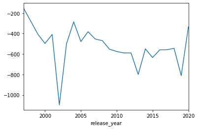
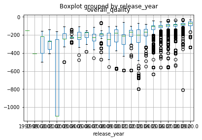
Electron Microscopy resolution has been said to be improving. Is this true? hint - the search term and filter can be different. pandas_plot_multi_groupby_min with use_min would be useful to plot this or maybe a box plot?
[34]:
search_terms = {'experimental_method':'Electron Microscopy'
               }
filter_results = ['resolution','release_year', 'pdb_id']
results = run_search(search_terms, filter_results, number_of_rows=1000000)
pandas_plot_multi_groupby_min(results, 'release_year', 'resolution', use_min=True)
pandas_box_plot(results, 'release_year', 'resolution')
https://www.ebi.ac.uk/pdbe/search/pdb/select?q=experimental_method:"Electron Microscopy"&fl=resolution,release_year,pdb_id&wt=json&rows=1000000
Number of results for Electron Microscopy: 47714
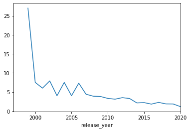
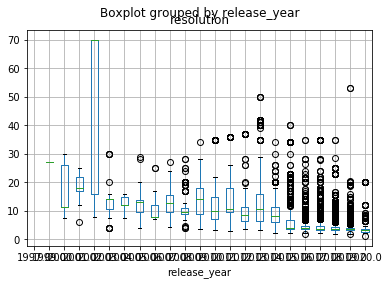
It has been said that all the simple structures have been done and that only complicated structures are left. One metric for “complicated” could be molecular weight.
[35]:
search_terms = {'experimental_method':'Electron Microscopy'
               }
filter_results = ['assembly_mol_wt','release_year', 'pdb_id']
results = run_search(search_terms, filter_results, number_of_rows=1000000)
pandas_box_plot(results, 'release_year', 'assembly_mol_wt')
https://www.ebi.ac.uk/pdbe/search/pdb/select?q=experimental_method:"Electron Microscopy"&fl=assembly_mol_wt,release_year,pdb_id&wt=json&rows=1000000
Number of results for Electron Microscopy: 47714
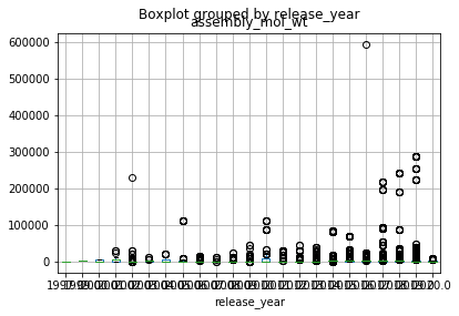
[ ]: